Rescale, Rotate, Shift and Warp, Warp from File Tools
Rescale
How to Rescale Tool in ArcToolbox ArcMap ArcGIS?? |
| Rescale Tool |
Path
to access the tool
:
Rescale Tool, Projections
and Transformations Toolset, Raster
Box, Data Management Tools Toolbox
Rescale
Resizes a raster by the
specified x and y scale factors.
1.
Input Raster
The input raster.
2.
Output Raster Dataset
Output raster dataset.
When storing the raster
dataset in a file format, you need to specify the file extension:
- .bil—Esri BIL
- .bip—Esri BIP
- .bmp—BMP
- .bsq—Esri BSQ
- .dat—ENVI DAT
- .gif—GIF
- .img—ERDAS IMAGINE
- .jpg—JPEG
- .jp2—JPEG 2000
- .png—PNG
- .tif—TIFF
- .mrf—MRF
- .crf—CRF
- No extension for Esri Grid
When storing a raster
dataset in a geodatabase, no file extension should be added to the name of the
raster dataset.
When storing your raster
dataset to a JPEG file, a JPEG 2000 file,
a TIFF file, or a geodatabase, you
can specify a Compression Type and Compression Quality in the geoprocessing
Environments.
3.
X Scale Factor
The factor in which to
scale the cell size in the x direction.
The factor must be
greater than zero.
4.
Y Scale Factor
The factor in which to
scale the cell size in the y direction.
The factor must be
greater than zero.
Rotate
How to Rotate Tool in ArcToolbox ArcMap ArcGIS??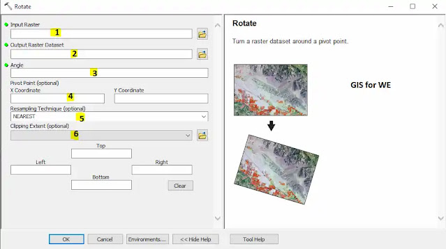 |
| Rotate Tool |
Path
to access the tool
:
Rotate Tool, Projections
and Transformations Toolset, Raster
Box, Data Management Tools Toolbox
Rotate
Turn a raster dataset
around a pivot point.
1.
Input Raster
Select the raster
dataset to rotate.
2.
Output Raster Dataset
Specify a name,
location, and format for the dataset you are creating. When storing a raster
dataset in a geodatabase, do not add a file extension to the name of the raster
dataset. When storing your raster dataset to a JPEG file, a JPEG 2000 file, a
TIFF file, or a geodatabase, you can specify a compression type and compression
quality.
When storing the raster
dataset in a file format, you need to specify the file extension:
- .bil—Esri BIL
- .bip—Esri BIP
- .bmp—BMP
- .bsq—Esri BSQ
- .dat—ENVI DAT
- .gif—GIF
- .img—ERDAS IMAGINE
- .jpg—JPEG
- .jp2—JPEG 2000
- .png—PNG
- .tif—TIFF
- .mrf—MRF
- .crf—CRF
- No extension for Esri Grid
3.
Angle
Specify a value between
0 and 360 degrees to rotate the raster by that amount in the clockwise
direction. To rotate the raster in the counterclockwise direction, specify the
angle as a negative value. The angle can be specified as an integer or a
floating-point value.
4.
Pivot Point (optional)
Select a point to rotate
the raster around. If left blank, the lower left corner of the input raster
dataset will serve as the pivot.
5.
Resampling Technique (optional)
The resampling algorithm
to be used. The default is NEAREST.
- NEAREST— Nearest neighbor is the fastest resampling method; it
minimizes changes to pixel values since no new values are created. It is
suitable for discrete data,
such as land cover.
- BILINEAR— Bilinear interpolation calculates the value of each
pixel by averaging (weighted for distance) the values of the surrounding four
pixels. It is suitable for continuous data.
- CUBIC— Cubic convolution calculates the value of each pixel by
fitting a smooth curve based on the surrounding 16 pixels. This produces the
smoothest image but can create values outside of the range found in the source
data. It is suitable for continuous data.
- MAJORITY—Majority resampling determines the value of each pixel
based on the most popular value in a 3 by 3 window. Suitable for discrete data.
The NEAREST and MAJORITY
options are used for categorical data, such as a land-use classification. The
NEAREST option is the default since it is the quickest and also because it will
not change the cell values. Do not use either of these for continuous data,
such as elevation surfaces.
The BILINEAR option and
the CUBIC option are most appropriate for continuous data. It is recommended
that neither of these be used with categorical data because the cell values may
be altered.
6.
Clipping Extent (optional)
Specify the processing
extent of the raster dataset. The source data will be clipped to the specified
extent before rotation.
Shift
How to Shift Tool in ArcToolbox ArcMap ArcGIS??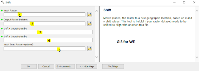 |
| Shift Tool |
Path
to access the tool
:
Shift Tool, Projections
and Transformations Toolset, Raster
Box, Data Management Tools Toolbox
Shift
Moves (slides) the
raster to a new geographic location, based on x and y shift values. This tool
is helpful if your raster dataset needs to be shifted to align with another
data file.
1.
Input Raster
The input raster
dataset.
2.
Output Raster Dataset
Output raster dataset.
When storing the raster
dataset in a file format, you need to specify the file extension:
- .bil—Esri BIL
- .bip—Esri BIP
- .bmp—BMP
- .bsq—Esri BSQ
- .dat—ENVI DAT
- .gif—GIF
- .img—ERDAS IMAGINE
- .jpg—JPEG
- .jp2—JPEG 2000
- .png—PNG
- .tif—TIFF
- .mrf—MRF
- .crf—CRF
- No extension for Esri Grid
When storing a raster
dataset in a geodatabase, no file extension should be added to the name of the
raster dataset.
When storing your raster
dataset to a JPEG file, a JPEG 2000 file, a TIFF file, or a geodatabase, you
can specify a Compression Type and Compression Quality in the geoprocessing
Environments.
3.
Shift X Coordinates by
The value used to shift
the x coordinates.
4.
Shift Y Coordinates by
The value used to shift
the y coordinates.
5.
Input Snap Raster (optional)
The raster dataset used
to align the cells of the output raster dataset.Input Snap Raster (optional)
Warp
How to Warp Tool in ArcToolbox ArcMap ArcGIS??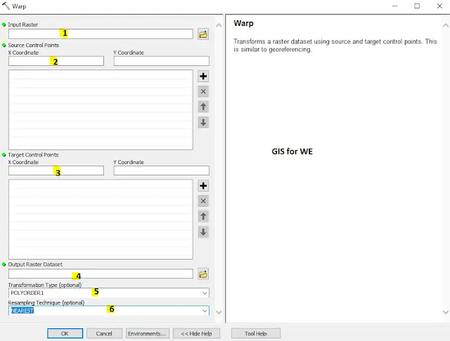 |
| Warp Tool |
Path
to access the tool
:
Warp Tool, Projections
and Transformations Toolset, Raster
Box, Data Management Tools Toolbox
Warp
Transforms a raster
dataset using source and target control points. This is similar to
georeferencing.
1.
Input Raster
The raster to be
transformed.
Source
Control Points
The coordinates of the raster to be warped.
Target
Control Points
The coordinates to which the source raster will be warped.
Output Raster
Dataset
Specify a name, location, and format for the dataset you are creating.
When storing a raster dataset in a geodatabase, do not add a file extension to
the name of the raster dataset. When storing your raster dataset to a JPEG
file, JPEG 2000 file, TIFF file, or geodatabase, you can specify a compression
type and compression quality.
When storing the raster dataset in a file format, you need to specify the
file extension:
· .bil—Esri BIL
· .bip—Esri BIP
· .bmp—BMP
· .bsq—Esri BSQ
· .dat—ENVI DAT
· .gif—GIF
· .img—ERDAS IMAGINE
· .jpg—JPEG
· .jp2—JPEG 2000
· .png—PNG
· .tif—TIFF
· .mrf—MRF
· .crf—CRF
· No extension for Esri Grid
Transformation
Type (optional)
Select a method for shifting the raster dataset.
· POLYORDER0— This method uses a zero-order polynomial to shift your data.
This is commonly used when your data is already georeferenced, but a small
shift will better line up your data. Only one link is required to perform a
zero-order polynomial shift.
· POLYSIMILARITY— This is a first order transformation that attempts to
preserve the shape of the original raster. The RMS error tends to be higher
than other polynomial transformations because the preservation of shape is more
important than the best fit.
· POLYORDER1—A first-order polynomial (affine) fits a flat plane to the
input points.
· POLYORDER2—A second-order polynomial fits a somewhat more complicated
surface to the input points.
· POLYORDER3—A third-order polynomial fits a more complicated surface to the
input points.
· ADJUST— This method combines a polynomial transformation and uses a
triangulated irregular network (TIN) interpolation technique to optimize for
both global and local accuracy.
· SPLINE— This method transforms the source control points precisely to the
target control points. In the output, the control points will be accurate, but
the raster pixels between the control points are not.
· PROJECTIVE— This method warps lines so they remain straight. In doing so,
lines that were once parallel may no longer remain parallel. The projective
transformation is especially useful for oblique imagery, scanned maps, and for
some imagery products.
Resampling
Technique (optional)
The resampling algorithm to be used. The default is NEAREST.
· NEAREST— Nearest neighbor is the fastest resampling method; it minimizes
changes to pixel values since no new values are created. It is suitable for
discrete data, such as land cover.
· BILINEAR— Bilinear interpolation calculates the value of each pixel by
averaging (weighted for distance) the values of the surrounding four pixels. It
is suitable for continuous data.
· CUBIC— Cubic convolution calculates the value of each pixel by fitting a
smooth curve based on the surrounding 16 pixels. This produces the smoothest
image but can create values outside of the range found in the source data. It
is suitable for continuous data.
· MAJORITY—Majority resampling determines the value of each pixel based on
the most popular value in a 3 by 3 window. Suitable for discrete data.
The NEAREST and MAJORITY options are used for categorical data, such as a
land-use classification. The NEAREST option is the default since it is the
quickest and also because it will not change the cell values. Do not use either
of these for continuous data, such as elevation surfaces.
The BILINEAR option and the CUBIC option are most appropriate for
continuous data. It is recommended that neither of these be used with
categorical data because the cell values may be altered.
2.
Source Control Points
The coordinates of the
raster to be warped.
Target
Control Points
The coordinates to which the source raster will be warped.
Output
Raster Dataset
Specify a name, location, and format for the dataset you are creating.
When storing a raster dataset in a geodatabase, do not add a file extension to
the name of the raster dataset. When storing your raster dataset to a JPEG
file, JPEG 2000 file, TIFF file, or geodatabase, you can specify a compression
type and compression quality.
When storing the raster dataset in a file format, you need to specify the
file extension:
· .bil—Esri BIL
· .bip—Esri BIP
· .bmp—BMP
· .bsq—Esri BSQ
· .dat—ENVI DAT
· .gif—GIF
· .img—ERDAS IMAGINE
· .jpg—JPEG
· .jp2—JPEG 2000
· .png—PNG
· .tif—TIFF
· .mrf—MRF
· .crf—CRF
· No extension for Esri Grid
Transformation
Type (optional)
Select a method for shifting the raster dataset.
· POLYORDER0— This method uses a zero-order polynomial to shift your data.
This is commonly used when your data is already georeferenced, but a small
shift will better line up your data.
Only one link is required to perform a
zero-order polynomial shift.
· POLYSIMILARITY— This is a first order transformation that attempts to
preserve the shape of the original raster. The RMS error tends to be higher
than other polynomial transformations because the preservation of shape is more
important than the best fit.
· POLYORDER1—A first-order polynomial (affine) fits a flat plane to the
input points.
· POLYORDER2—A second-order polynomial fits a somewhat more complicated
surface to the input points.
· POLYORDER3—A third-order polynomial fits a more complicated surface to the
input points.
· ADJUST— This method combines a polynomial transformation and uses a
triangulated irregular network (TIN) interpolation technique to optimize for
both global and local accuracy.
· SPLINE— This method transforms the source control points precisely to the
target control points. In the output, the control points will be accurate, but
the raster pixels between the control points are not.
· PROJECTIVE— This method warps lines so they remain straight. In doing so,
lines that were once parallel may no longer remain parallel. The projective
transformation is especially useful for oblique imagery, scanned maps, and for
some imagery products.
Resampling
Technique (optional)
The resampling algorithm to be used. The default is NEAREST.
· NEAREST— Nearest neighbor is the fastest resampling method; it minimizes
changes to pixel values since no new values are created. It is suitable for
discrete data, such as land cover.
· BILINEAR— Bilinear interpolation calculates the value of each pixel by
averaging (weighted for distance) the values of the surrounding four pixels. It
is suitable for continuous data.
· CUBIC— Cubic convolution calculates the value of each pixel by fitting a
smooth curve based on the surrounding 16 pixels. This produces the smoothest
image but can create values outside of the range found in the source data. It
is suitable for continuous data.
· MAJORITY—Majority resampling determines the value of each pixel based on
the most popular value in a 3 by 3 window. Suitable for discrete data.
The NEAREST and MAJORITY options are used for categorical data, such as a
land-use classification. The NEAREST option is the default since it is the
quickest and also because it will not change the cell values. Do not use either
of these for continuous data, such as elevation surfaces.
The BILINEAR option and the CUBIC option are most appropriate for
continuous data. It is recommended that neither of these be used with
categorical data because the cell values may be altered.
3.
Target Control Points
The coordinates to which
the source raster will be warped.
Output
Raster Dataset
Specify a name, location, and format for the dataset you are creating.
When storing a raster dataset in a geodatabase, do not add a file extension to
the name of the raster dataset. When storing your raster dataset to a JPEG
file, JPEG 2000 file, TIFF file, or geodatabase, you can specify a compression
type and compression quality.
When storing the raster dataset in a file format, you need to specify the
file extension:
· .bil—Esri BIL
· .bip—Esri BIP
· .bmp—BMP
· .bsq—Esri BSQ
· .dat—ENVI DAT
· .gif—GIF
· .img—ERDAS IMAGINE
· .jpg—JPEG
· .jp2—JPEG 2000
· .png—PNG
· .tif—TIFF
· .mrf—MRF
· .crf—CRF
· No extension for Esri Grid
Transformation
Type (optional)
Select a method for shifting the raster dataset.
· POLYORDER0— This method uses a zero-order polynomial to shift your data.
This is commonly used when your data is already georeferenced, but a small
shift will better line up your data. Only one link is required to perform a
zero-order polynomial shift.
· POLYSIMILARITY— This is a first order transformation that attempts to
preserve the shape of the original raster. The RMS error tends to be higher than
other polynomial transformations because the preservation of shape is more
important than the best fit.
· POLYORDER1—A first-order polynomial (affine) fits a flat plane to the
input points.
· POLYORDER2—A second-order polynomial fits a somewhat more complicated
surface to the input points.
· POLYORDER3—A third-order polynomial fits a more complicated surface to the
input points.
· ADJUST— This method combines a polynomial transformation and uses a
triangulated irregular network (TIN) interpolation technique to optimize for
both global and local accuracy.
· SPLINE— This method transforms the source control points precisely to the
target control points. In the output, the control points will be accurate, but
the raster pixels between the control points are not.
· PROJECTIVE— This method warps lines so they remain straight. In doing so,
lines that were once parallel may no longer remain parallel. The projective
transformation is especially useful for oblique imagery, scanned maps, and for
some imagery products.
Resampling
Technique (optional)
The resampling algorithm to be used. The default is NEAREST.
· NEAREST— Nearest neighbor is the fastest resampling method; it minimizes
changes to pixel values since no new values are created. It is suitable for
discrete data, such as land cover.
· BILINEAR— Bilinear interpolation calculates the value of each pixel by averaging
(weighted for distance) the values of the surrounding four pixels. It is
suitable for continuous data.
· CUBIC— Cubic convolution calculates the value of each pixel by fitting a
smooth curve based on the surrounding 16 pixels. This produces the smoothest
image but can create values outside of the range found in the source data. It
is suitable for continuous data.
· MAJORITY—Majority resampling determines the value of each pixel based on
the most popular value in a 3 by 3 window. Suitable for discrete data.
The NEAREST and MAJORITY options are used for categorical data, such as a
land-use classification. The NEAREST option is the default since it is the
quickest and also because it will not change the cell values. Do not use either
of these for continuous data, such as elevation surfaces.
The BILINEAR option and the CUBIC option are most appropriate for
continuous data. It is recommended that neither of these be used with
categorical data because the cell values may be altered.
4.
Output Raster Dataset
Specify a name,
location, and format for the dataset you are creating. When storing a raster
dataset in a geodatabase, do not add a file extension to the name of the raster
dataset. When storing your raster dataset to a JPEG file, JPEG 2000 file, TIFF
file, or geodatabase, you can specify a compression type and compression
quality.
When storing the raster
dataset in a file format, you need to specify the file extension:
.bil—Esri BIL- .bip—Esri BIP
- .bmp—BMP
- .bsq—Esri BSQ
- .dat—ENVI DAT
- .gif—GIF
- .img—ERDAS IMAGINE
- .jpg—JPEG
- .jp2—JPEG 2000
- .png—PNG
- .tif—TIFF
- .mrf—MRF
- .crf—CRF
- No extension for Esri Grid
5.
Transformation Type (optional)
Select a method for
shifting the raster dataset.
- POLYORDER0— This method uses a zero-order polynomial to shift your
data. This is commonly used when your data is already georeferenced, but a
small shift will better line up your data. Only one link is required to perform
a zero-order polynomial shift.
- POLYSIMILARITY— This is a first order transformation that attempts
to preserve the shape of the original raster. The RMS error tends to be higher
than other polynomial transformations because the preservation of shape is more
important than the best fit.
- POLYORDER1—A first-order polynomial (affine) fits a flat plane to
the input points.
- POLYORDER2—A second-order polynomial fits a somewhat more
complicated surface to the input points.
- POLYORDER3—A third-order polynomial fits a more complicated
surface to the input points.
- ADJUST— This method combines a polynomial transformation and uses a
triangulated irregular network (TIN) interpolation technique to optimize for
both global and local accuracy.
- SPLINE— This method transforms the source control points precisely
to the target control points. In the output, the control points will be accurate,
but the raster pixels between the control points are not.
- PROJECTIVE— This method warps lines so they remain straight. In
doing so, lines that were once parallel may no longer remain parallel. The
projective transformation is especially useful for oblique imagery, scanned
maps, and for some imagery products.
Resampling
Technique (optional)
The resampling algorithm to be used. The default is NEAREST.
· NEAREST— Nearest neighbor is the fastest resampling method; it minimizes
changes to pixel values since no new values are created. It is suitable for
discrete data, such as land cover.
· BILINEAR— Bilinear interpolation calculates the value of each pixel by averaging
(weighted for distance) the values of the surrounding four pixels. It is
suitable for continuous data.
· CUBIC— Cubic convolution calculates the value of each pixel by fitting a
smooth curve based on the surrounding 16 pixels. This produces the smoothest
image but can create values outside of the range found in the source data. It
is suitable for continuous data.
· MAJORITY—Majority resampling determines the value of each pixel based on
the most popular value in a 3 by 3 window. Suitable for discrete data.
The NEAREST and MAJORITY options are used for categorical data, such as a
land-use classification. The NEAREST option is the default since it is the
quickest and also because it will not change the cell values. Do not use either
of these for continuous data, such as elevation surfaces.
The BILINEAR option and the CUBIC option are most appropriate for
continuous data. It is recommended that neither of these be used with
categorical data because the cell values may be altered.
6.
Resampling Technique (optional)
The resampling algorithm
to be used. The default is NEAREST.
- NEAREST— Nearest neighbor is the fastest resampling method; it
minimizes changes to pixel values since no new values are created. It is
suitable for discrete data, such as land cover.
- BILINEAR— Bilinear interpolation calculates the value of each
pixel by averaging (weighted for distance) the values of the surrounding four
pixels. It is suitable for continuous data.
- CUBIC— Cubic convolution calculates the value of each pixel by
fitting a smooth curve based on the surrounding 16 pixels. This produces the
smoothest image but can create values outside of the range found in the source
data. It is suitable for continuous data.
- MAJORITY—Majority resampling determines the value of each pixel
based on the most popular value in a 3 by 3 window. Suitable for discrete data.
The NEAREST and MAJORITY
options are used for categorical data, such as a land-use classification. The
NEAREST option is the default since it is the quickest and also because it will
not change the cell values. Do not use either of these for continuous data,
such as elevation surfaces.
The BILINEAR option and
the CUBIC option are most appropriate for continuous data. It is recommended
that neither of these be used with categorical data because the cell values may
be altered.
Warp from File
How to Warp from File Tool in ArcToolbox ArcMap ArcGIS??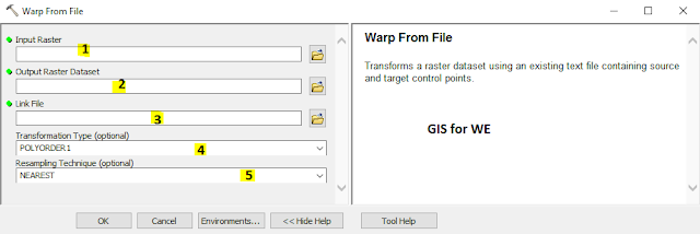 |
| Warp from File |
Path
to access the tool
:
Warp
from File Tool, Projections
and Transformations Toolset, Raster
Box, Data Management Tools Toolbox
Warp from File
Transforms a raster
dataset using an existing text file containing source and target control
points.
1.
Input Raster
The raster that you want
to transform.
Output
Raster Dataset
The name, location, and format for the dataset you are creating. When
storing a raster dataset in a geodatabase, do not add a file extension to the
name of the raster dataset. When storing your raster dataset to a JPEG file, a
JPEG 2000 file, a TIFF file, or a geodatabase, you can specify a compression
type and compression quality using environment settings.
· .bil—Esri BIL
· .bip—Esri BIP
· .bmp—BMP
· .bsq—Esri BSQ
· .dat—ENVI DAT
· .gif—GIF
· .img—ERDAS IMAGINE
· .jpg—JPEG
· .jp2—JPEG 2000
· .png—PNG
· .tif—TIFF
· .mrf—MRF
· .crf—CRF
· No extension for Esri Grid
Link File
The text, CSV, or TAB file containing the coordinates to warp the input
raster. This can be generated from the Register Raster tool or from the
Georeferencing toolbar.
Transformation
Type (optional)
Select a method for shifting the raster dataset.
· POLYORDER0— This method uses a zero-order polynomial to shift your data.
This is commonly used when your data is already georeferenced, but a small
shift will better line up your data. Only one link is required to perform a
zero-order polynomial shift.
· POLYSIMILARITY— This is a first order transformation that attempts to
preserve the shape of the original raster. The RMS error tends to be higher
than other polynomial transformations because the preservation of shape is more
important than the best fit.
· POLYORDER1—A first-order polynomial (affine) fits a flat plane to the
input points.
· POLYORDER2—A second-order polynomial fits a somewhat more complicated
surface to the input points.
· POLYORDER3—A third-order polynomial fits a more complicated surface to the
input points.
· ADJUST— This method combines a polynomial transformation and uses a
triangulated irregular network (TIN) interpolation technique to optimize for
both global and local accuracy.
· SPLINE— This method transforms the source control points precisely to the
target control points. In the output, the control points will be accurate, but
the raster pixels between the control points are not.
· PROJECTIVE— This method warps lines so they remain straight. In doing so,
lines that were once parallel may no longer remain parallel. The projective
transformation is especially useful for oblique imagery, scanned maps, and for
some imagery products.
Resampling
Technique (optional)
Choose an appropriate technique based on the type of data you have.
· NEAREST— Nearest neighbor is the fastest resampling method; it minimizes
changes to pixel values since no new values are created. It is suitable for
discrete data, such as land cover.
· BILINEAR— Bilinear interpolation calculates the value of each pixel by averaging
(weighted for distance) the values of the surrounding four pixels. It is
suitable for continuous data.
· CUBIC— Cubic convolution calculates the value of each pixel by fitting a
smooth curve based on the surrounding 16 pixels. This produces the smoothest
image but can create values outside of the range found in the source data. It
is suitable for continuous data.
· MAJORITY—Majority resampling determines the value of each pixel based on
the most popular value in a 3 by 3 window. Suitable for discrete data.
The NEAREST and MAJORITY options are used for categorical data, such as a
land-use classification. The NEAREST option is the default since it is the
quickest and also because it will not change the cell values. Do not use either
of these for continuous data, such as elevation surfaces.
The BILINEAR option and the CUBIC option are most appropriate for
continuous data. It is recommended that neither of these be used with
categorical data because the cell values may be altered.
2.
Output Raster Dataset
The name, location, and
format for the dataset you are creating. When storing a raster dataset in a
geodatabase, do not add a file extension to the name of the raster dataset.
When storing your raster dataset to a JPEG file, a JPEG 2000 file, a TIFF file,
or a geodatabase, you can specify a compression type and compression quality
using environment settings.
- .bil—Esri BIL
- .bip—Esri BIP
- .bmp—BMP
- .bsq—Esri BSQ
- .dat—ENVI DAT
- .gif—GIF
- .img—ERDAS IMAGINE
- .jpg—JPEG
- .jp2—JPEG 2000
- .png—PNG
- .tif—TIFF
- .mrf—MRF
- .crf—CRF
- No extension for Esri Grid
3.
Link File
The text, CSV, or TAB
file containing the coordinates to warp the input raster. This can be generated
from the Register Raster tool or from the Georeferencing toolbar.
4.
Transformation Type (optional)
Select a method for
shifting the raster dataset.
- POLYORDER0— This method uses a zero-order polynomial to shift your
data. This is commonly used when your data is already georeferenced, but a
small shift will better line up your data. Only one link is required to perform
a zero-order polynomial shift.
- POLYSIMILARITY— This is a first order transformation that attempts
to preserve the shape of the original raster. The RMS error tends to be higher
than other polynomial transformations because the preservation of shape is more
important than the best fit.
- POLYORDER1—A first-order polynomial (affine) fits a flat plane to
the input points.
- POLYORDER2—A second-order polynomial fits a somewhat more
complicated surface to the input points.
- POLYORDER3—A third-order polynomial fits a more complicated
surface to the input points.
- ADJUST— This method combines a polynomial transformation and uses
a triangulated irregular network (TIN) interpolation technique to optimize for
both global and local accuracy.
- SPLINE— This method transforms the source control points precisely
to the target control points. In the output, the control points will be
accurate, but the raster pixels between the control points are not.
- PROJECTIVE— This method warps lines so they remain straight. In
doing so, lines that were once parallel may no longer remain parallel. The
projective transformation is especially useful for oblique imagery, scanned
maps, and for some imagery products.
5.
Resampling Technique (optional)
Choose an appropriate
technique based on the type of data you have.
- NEAREST— Nearest neighbor is the fastest resampling method; it
minimizes changes to pixel values since no new values are created. It is
suitable for discrete data, such as land cover.
- BILINEAR— Bilinear interpolation calculates the value of each
pixel by averaging (weighted for distance) the values of the surrounding four
pixels. It is suitable for continuous data.
- CUBIC— Cubic convolution calculates the value of each pixel by
fitting a smooth curve based on the surrounding 16 pixels. This produces the
smoothest image but can create values outside of the range found in the source
data. It is suitable for continuous data.
- MAJORITY—Majority resampling determines the value of each pixel
based on the most popular value in a 3 by 3 window. Suitable for discrete data.
The NEAREST and MAJORITY
options are used for categorical data, such as a land-use classification. The
NEAREST option is the default since it is the quickest and also because it will
not change the cell values. Do not use either of these for continuous data,
such as elevation surfaces.
The BILINEAR option and
the CUBIC option are most appropriate for continuous data. It is recommended
that neither of these be used with categorical data because the cell values may
be altered.


Comments
Post a Comment